Solution Manual For Introduction To Engineering Experimentation, 3rd Edition

Preview (31 of 298 Pages)

100%

Purchase to unlock

Loading page image...

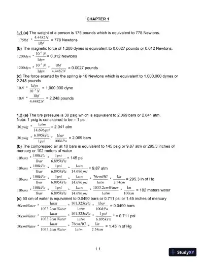
1.1CHAPTER 11.1(a)The weight of a person is 175 pounds which is equivalent to 778 Newtons.lbf175*lbfN14482.4= 778 Newtons(b)The magnetic force of 1,200 dynes is equivalent to 0.0027 pounds or 0.012 Newtons.dyn1200*dynN1105−= 0.012 Newtonsdyn1200*dynN1105−*Nlbf4482.41= 0.0027 pounds(c)The force exerted by the spring is 10 Newtons which is equivalent to 1,000,000 dynes or2.248 poundsN10*Ndyn5101−= 1,000,000 dyneN10*Nlbf4482.41= 2.248 pounds1.2(a)The tire pressure is 30 psig which is equivalent to 2.069 bars or 2.041 atm.Note:1psig is considered to be =1psipsig30*psiatm696.141= 2.041 atmpsig30*psikPa1895.6*kPabar1001= 2.069 bars(b)The compressed air at 10 bars is equivalent to 145 psig or 9.87 atm or 295.3 inches ofmercury or 102 meters of waterbars10*barkPa1100*kPapsi895.61= 145 psibars10*barkPa1100*kPapsi895.61*psiatm696.141= 9.87 atmbars10*barkPa1100*kPapsi895.61*psiatm696.141*atmcmHG176*cmin54.21= 295.3 in of Hgbars10*barkPa1100*kPapsi895.61*psiatm696.141*atmcmWater12.1033*cmm1001= 102 meters water(c)50 cm of water is equivalent to 0.0490 bars or 0.711 psi or 1.45 inches of mercurycmWater50*cmWateratm2.10331*atmkPa1325.101*kPabar1001= 0.0490 barscmWater50*cmWateratm2.10331*atmkPa1325.101*kPapsi895.61* = 0.711 psicmWater50*cmWateratm2.10331*atmcmHG176*cmin54.21= 1.45 in of Hg

Loading page image...

1.21.3(a)The household energy use of 750 kWh is equivalent to 2,559,241.71 Btu or 645,007kCal or 2,700,000,000 jouleskWh750*kWhkJ13600*kJJ11000*JBtu10551= 2,559,241.71 BtukWh750*kWhkJ13600*kJJ11000*Jcal186.41*calkcal10001= 645,007 kcalkWh750*kWhkJ13600*kJJ11000= 2,700,000,000 J(b)The gas water heater uses 50,000 Btu or 52,750,000 joules or 12,601.5 kcal or38,908,386 ft.lbfBtu50000*BtuJ11055= 52,750,000 joulesBtu50000*BtuJ11055*Jcal186.41*calkcal10001= 12,601.5 kcalBtu50000*Btulbfft00128507.0.1= 38,908,386 ft.lbf(c)The amount of heat required is 250 kCal which is equivalent to 992 Btu or 250,000 Calor 1,046,500 jouleskcal250*kcalcal11000*calJ1186.4*JBtu10551= 992 Btukcal250*kcalcal11000= 250,000 calkcal250*kcalcal11000*calJ1186.4= 1,046,500 J

Loading page image...

1.31.4(a)The automobile rating of 150 hp is equivalent to 112 kW or 82,500 ft.lbf/sec or106.02 Btu/sechp150*hpW17.745*WkW10001= 112 kWhp150*hpslbfft1.550= 82,500 ft.lbf/sechp150*hpW17.745*WsBtu04.10551= 106.02 Btu/sec(b)The truck rating of 400 kW is equivalent to 536 hp or 295,025 ft.lbf/sec or 379 Btu/seckW400*kWW11000*Whp7.7451= 536 hpkW400*kWW11000*Whp7.7451*hpslbfft1.550= 295,025 ft.lbf/seckW400*kWW11000*WsBtu04.10551= 379 Btu/sec(c)The water heater rating of 40,000 Btu/hr is equivalent to 11.72 kWhrBtu40000*hrBtuW1293.0*WkW10001= 11.72 kW

Loading page image...

1.41.5(a)50oF is equivalent to 10oC(95)(50–32) = 10oC(b)150oC is equivalent to 302oF(59)(150oC) + 32 = 302oF(c)The water temperature increase of 40oC is equivalent to a change of 40 K or 72oF or 72oR(40oC) *CK11= 40 K(40oC) *CF18.1= 72oF(40oC) *CR18.1= 72oR(d)The air temperature change of 30oF is equivalent to a change of 16.7 K or 16.7oC or 30oR(30oF) *FK1556.0= 16.7 K(30oF) *FC1556.0= 16.7oC(30oF) *FR11= 30oR

Loading page image...

1.51.6(a)4 gallons is equivalent to 15.1 liter or 15,142 cm3or 0.535 ft3gal4*galm10037854.03*33101mLiter−= 15.1 litergal4*galm10037854.03*363101mcm−= 15,142 cm3gal4*gal10037854.0*3302832.01mft= 0.535 ft3(b)10 liters is equivalent to 2.64 gallons or 10,000 cm3or 0.353 ft3Liter10*literm11033−*30037854.01mgal= 2.64 gallonsLiter10*literm11033−*363101mcm−= 10,000 cm3Liter10*literm11033−*3302832.01mft= 0.353 ft3(c)5 ft3is equivalent to 37.4 gallons or 141,600 cm3or 142 liters35ft*313368.01ftgal= 37.4 gallons35ft*33102832.0ftm*363101mcm−= 141,600 cm335ft*33102832.0ftm*33101mliter−= 142 liters1.7The air gas constant of 53.34 ft.lbf/lbm.oR is equivalent to 0.0685 Btu/lbm.oR or 287joules/kg.K or 0.0686 kcal/kg.KRlbmlbfft.34.53*lbfftBtu.100128507.0= 0.0685 Btu/lbm.oRRlbmlbfft.34.53*lbfftBtu.100128507.0*BtuJ11055*kglbm4536.01*KR951= 287 J/kg.KRlbmlbfft.34.53*lbfftBtu.100128507.0*BtuJ11055*Jcal186.41*calkcal10001*kglbm4536.01*KR951=Kkgkcal0685.0

Loading page image...

1.61.8The universal gas constant is 1.986 Btu/lb mole.oR which is equivalent to 1.986 kCal.kgmole.K or 1,545 ft.lbf/lb mole.oR or 8,314 joules/kg mole.KRlbmoleBtu986.1*BtuJ11055*Jcal186.41*calkcal10001*kglbm4536.01*KR951= 1.986 kCal.kg mole.KRlbmoleBtu986.1*Btulbfft00128507.0.1= 1,545 ft.lbf/lb mole.oRRlbmoleBtu986.1*BtuJ11055*kglbm4536.01*KR951= 8,314 J/kg mole.K1.9The thermal conductivity is 200 W/m.oC or 116 Btu/hr/ft/oF or 0.048 kcal/sec.m.oCCmW200*CmWFfthrBtu7307.1..1= 116 Btu/hr/ft/oFCmW200*WsBtu04.10551*BtuJ11055*Jcal186.41*calkcal10001= 0.048 kcal/sec.m.oC1.10The thermal conductivity is 50 Btu/hr.ft.oF or 86.54 W/m.oC or 20.7 Cal/sec.m.oCFfthrBtu.50*FfthrBtuCmW.17307.1= 86.54 W/m.oCFfthrBtu.50*FfthrBtuCmW.17307.1*WsBtu04.10551*BtuJ11055*Jcal186.41= 20.7 cal/sec.m.oC

Loading page image...

2.1CHAPTER 22.1(a)The mechanical speedometer measures vehicle speed by measuring the angularvelocity of the wheels. The angular velocity of the wheels (through some gears) causes aflexible cable to rotate. This cable causes a magnet to rotate inside a metal cup creating acircumferential drag on the cup (a torque). The drag is sensed by allowing the cup to rotateless than a complete turn against the resistance of a torsional spring. The cup is connectedto a pointer which can be compared to a stationary scale.The sensing element is the magnet rotating inside the metal cup creating drag. The signalmodification system is the system that allows the cup to rotate against a torsional spring.The indicator is the comparison of the pointer to a stationary scale.(b)The fuel level inside a fuel tank is measured with a mechanical float which follows thesurface of the fuel (see Ch. 10). The position of the float is sensed with a connected armwhich rotates a rotary variable resistor (angular potentiometer, see Ch. 8). The resistanceof the variable resistor is sensed by passing applying a voltage to the resistor andmeasuring the current with an electromechanical gage. The sensing element is the float.The signal modification system consists of the angular potentiometer and the indicator is theelectromechanical gage.(c)Most of these devices use a variable resistance device called a thermistor. Theresistance of the thermistor is a strong function of it’s temperature. The resistance issensed by passing applying a voltage to the device and sensing the current, which will be afunction of temperature. The current is then converted to a digital form which is then outputto the display. In this case, the thermistor is the sensing device. The signal modificationsystem is quite complicated including the creation of the current and the conversion todigital form. Finally, the indicator is the liquid crystal display.WheelGearsFlexCableRot.MagnetCupPointer

Loading page image...

2.22.2True Value = 0.5000 inchesDetermination of Bias Error.First, the average of readings must be calculated:Average of Readings =in4821.048214.010/)4822.04820.04822.04821.04822.04820.04821.04821.04824.04821.0(==+++++++++Bias Error = Average of Readings-True Value=−= −= −0 48210 50000 017860 0179....inDetermination of Maximum Precision Error:Maximum Precision Error =Largest difference between a singlereading and the Average of Readings=−=0 48240 48210 0003...in2.3Readings:20.2, 20.2, 20.6, 20.0, 20.4, 20.2, 20.0, 20.6, 20.0, 20.2 (lb)First determine the average of the reading:Average W = 20.2 lbFor bias error,Bias Error = Average Value-True Value= 20.24-20.0= 0.2 lbFor maximum precision error, we need the reading with the greatest deviation fromthe average reading (20.6 lb). Therefore,Maximum Precision Error = 20.6-20.2 = 0.4 lb2.4(a)Intrusive; The thermometer causes a loading error.(b)Non-intrusive; The photography does not affect the speed of the bullet at any time.(c)Non-intrusive; Optical thermal radiation device would yield a non-intrusive measurementas long as it is insulated from the furnace.(d)Non-intrusive; The speed of the car is unaffected by waves measured by the radar gun.

Loading page image...

2.32.5(a)A single conducting wire induces a small magnetic field around itself and if it isalternating current, will induce an alternating magnetic in the clamp on ammeter. The clampon ammeter will have a negligible effect on the current in the wire and for all practicalpurposes is non-intrusive.(b)The orifice meter (see Ch.10) measures fluid flowrate by obstructing the flow in pipe andmeasuring the resultant pressure drop. The pressure drop is significant and this device isintrusive.(c)This device passes a beam of infrared radiation through the gases which absorb some ofthe radiation (see Ch. 10). This measurement has no effect on the composition of the gasesand negligible effect on the gas temperature. It is non-intrusive.(d)This device measures rotational speed by shining a pulsing light on a mark on the shaftand adjusting the pulsing rate until the mark appears stationary (see Ch. 8). The light hasnegligible effect on the rotation of the shaft and is non-intrusive.2.6(a)Bias Error; The output will consistently deviate from the true value.(b)Precision Error; The speedometer output shows data scatter.(c)If the difference is consistent with time, then it is a bias error-either of calibration orspatial error. If the difference varies with time, it is precision.2.7(a)In most cases, this error will by systematic since repeated measurements at thesame time will produce the same error. However, if measurements are made over a longperiod of time and the temperature varies randomly, the error will be random.(b)This error will be the same each time the measurement is made by the same personwith the same procedure and hence is systematic. However, if the measurement is made byseveral people using different procedures, it may appear to be random.(c)This error will be the same each time the measurement is made and is alwayssystematic.2.8(a)This error is usually considered systematic if the readings are all made at the sameambient temperature. However, if the readings are taken over a period of time and theambient temperature varies randomly, then the error will appear random.(b)This is always random since the fields normally vary in a random manner.(c)Since this is a malfunction, it is not predictable in occurrence so it would be consideredrandom.2.9(a)This error is usually considered random even if the readings are all made at thesame conditions since corn-growing conditions are highly dependent on various factors.(b)The deterioration of asphalt/concrete in a highway is a combination of factors that needsfurther analysis since the same-grade concrete will deteriorate at a same rate which gives asystematic error, but given the various conditions at which the different portions of thehighway is exposed to the elements, each section will have a random error.(c)The variation of height of the same type of tree in an orchard qualifies as a random errorsince the height of each tree is highly dependent various growth factors.(d)The variation of drying time of concrete columns of a highway is subjected to bothsystematic and random error; only if the drying conditions are constant for all columns andthe concrete grade is uniform throughout the highway will the error be limited to systematic.

Loading page image...

2.42.10(a)The variation in access for a popular website would usually be considered arandom error since it is dependent on unknown factors.(b)The variation in average access per day of a popular website would also be considereda random error since it is due to uncontrollable factors.(c)The variation in the rider-ship of a bus or train line would usually be considered arandom error since it is dependent on unknown factors.(d)The variation in the rider-ship of a bus or train would also be considered a random errorsince it is due to uncontrollable factors.2.11Resolution or readability does not necessarily give any information about accuracy sowe cannot make any statement about accuracy. However, the digital device can be read toonly 1 part in 999 of the full scale reading. It may be possible to interpolate betweendivisions on the analog device giving an effective resolution that is better.2.12The span is 50-0 = 50 m/s.2.13(a)The span is 50-5 = 45 psig(b)70 cm vacuum is taken to be 70 cm of mercury which is equivalent to 93 kPa. Thus, thespan is 200-93 = 107 kPa(c)The span is 150-10 = 140 kPa2.14Device (D) would be the best. Device (C) is really the closest in its range. However,measurement errors might cause device (C) to be over range for some measurementsproducing meaningless results.2.15Manufacturer Accuracy =2.0% of full scale=0.02(30V)=0.6V% uncertainty of accuracy =(0.6V/5V)(100) =12%The resolution of the device is 0.1 Volts. With a reading of 5V,% uncertainty of resolution = (0.1V/5V)(100) = 2% (or1%)2.16(a)The maximum reading for each range will be 2.999, 29.99, 299.9 and 2999. and theresolution uncertainty will be 1 in the least significant digit. So the resolution uncertainty willbe 0.001V, ).01V, 0.1V and 1V for the three ranges. This could also be viewed as0.0005V,0.005V,0.05V and0.5V(b)The uncertainties will be 2% of full scale. This is .02*3 for the lowest scale or0.06V.Similarly for the higher ranges, the uncertainties will be0.6V,6V and60V.(c)The resolution uncertainty is negligible compared to the accuracy. Hence we can use theresults of part (b). For the 30 V range the relative uncertainy will be 0.06/25 =2.4%. Forthe higher ranges, the uncertainties are24% and240%.

Loading page image...

2.52.17Since the device reads 0.5 psi when it should read zero, it has a zero offset of 0.5 psiwhich will affect all readings. Zero offset is not a component of accuracy. The accuracyspecification of 0.2% of full scale gives an uncertainty of0.00250 =0.1 psi. This meansthat we can have an expected error in any reading of 0.50.1 psi. For an applied pressure of20 psi, the reading would be expected to be in the range 20.4 to 20.6 psi.We can reduce the expected error by either adjusting the zero (if possible) or by subtracting0.5 psi from each reading. It may be possible to reduce the error due to the accuracyspecification by a calibration of the gage.2.18With 2V reading when leads are shorted together,Error 1 = 2VError 2 =4%(100) =4VMaximum Total Error = +6/-2V = (6V/80V)(100) = +7.5%With 0V reading when leads are shorted together,Error =4%(100) =4VMaximum Percent Error =(4V/80V)(100) =5%2.19The range of both temperature gages will allow the intended 300 C measurement. Theuncertainty for each of the two gages is 2% of its span; this gives an uncertainty of 8 C and18 C for the temperature gage with the smaller and larger span respectively. Thus, thetemperature gage with range of 100 C to 500 C should be selected since there is smalleruncertainty.2.20The sensitivity isoutput/input. This is (125-5)/1000-100) = 0.1333 mV/kPa.2.21The sensitivity isoutput/input. This is (150-10)/100-10) = 1.556 mV/psi2.22The relationship between pressure and temperature is given by:PVmRTPmRTV==The sensitivity is given by:dPdTmRVPTR m and V constii==;,,tanWe see the sensitivitydPdTis proportional to the initial pressure and is changed when theinitial filling pressure is changed.2.23(a)The sensitivity from A to C is not a constant and gets smaller from A to C.(b)If a high degree of sensitivity is required, use A-B. For most purposes, B-C would notbe recommended due to the sensitivity approaching zero at C.2.24Usually, the maximum output increases proportionally with increasing range so thesensitivity will be unchanged.2.25Installing an amplifier will increase the sensitivity.

Loading page image...

2.62.26(a)For this device, the output isP and the input is Q. So the sensitivity is simply thederivative ofP with respect to Q. Solving forP we get:2=CQPthen22CQdQPd=(b)The sensitivity increases with flowrate and with pressure drop.(c)This device is best for values ofP which are high relative to the design value. At 10% ofthe design Q, the pressure drop will be only 1% of the design pressure drop.2.27Ideal sensitivity = 0.1 cm/NInput span = 200 NIdeal output span = Input spanIdeal Sensitivity= 200N0.1cm/N= 20 cmActual sensitivity = 0.105 cm/NActual output span = Input spanActual sensitivity= 200N0.105cm/N=21 cm%error of output span =()ActualIdealIdeal−100()=−=2120201005%

Loading page image...

2.72.28020406080100120Gage Reading - psi020406080100True Pressure - psiPlot of Data for Problem 2.13The best fit line is:Reading = 2.9 + 0.978 (True Pressure)psiTrueDeviation (Readings-Best Fit) (psi)Pressure(psi)Cycle 1Cycle 2Cycle 3Cycle 4Cycle 520-2-3-2-2-340-3-2-3-3-360-3-4-3-4-280-1-1-2-2-11000-1-1018032333601110040101122022222021131The accuracy can be evaluated from the extreme deviation values. The values are +3 and-4 psi. For a span of 100 psi, these values result in an accuracy of +3% and-4% of full scale.The repeatability can be evalued from Table P2.13 in the problem statement. The maximumdeviation for a given measurand and direction is 2 psi. The repeatability can then beexpressed as1% of full scale.Hysteresis is the maximum difference between the up and down readings for anymeasurand value in the same calibration cycle. The maximum difference is 5 psi, occuringseveral times (Cycle 2, 20 psi is an example). This can be expressed as 5% of span.-4-3-2-10123Reading minus Best Fit - psi020406080100True Pressure - psiDeviation Data for Problem 2.13

Loading page image...

2.82.29-200020040060080010001200Gage Reading -kPa02004006008001000True Pressure - kPaPlot of Data for Problem 2.14Best FitLineBest Fit Line:Reading =-4.5 + 1.017 (True Pressure)Deviations based on difference between readings and best fit line.TrueDeviations (Readings-Best Fit) (N)Force(N)Cycle 1Cycle 2Cycle 3Cycle 4Cycle 5200-7-8-5-6-7400-11-13-11-10-9600-10-9-9-13-10800-2-3-4-6-4100010109108800757786000-3-3-3-2400-310-112004231601517141615The accuracy can be determined from the deviation data. The maximum positive deviationis 17 Pa and the largest negative deviation is-13 Pa. For a span of 1000 Pa, this translatesto an accuracy of +1.7% and-1.3% of full scale. Note: this accuracy only applies when thereadings are corrected using the above curve fit to the data.The repeatability can be evaluated from the deviations given in Table P2.14. This occurs atthe 200 Pa "down" reading and has a value of 5 Pa. This translates to0.5% of full scale.The hysteresis error is given by the maximum deviation between the up and the downreadings for any value of the measurand in one cycle. The value is 14 Pa which occurs at400 Pa in Cycle 2.-15-10-505101520Reading minus02004006008001000True Pressure -k PaDeviation Data for Problem 2.14Best Fit - kPa

Loading page image...

2.92.30-1001020304050Output - mV020406080100Force - NPlot of Data for Problem 2.15Best FitLineEquations of the best fit line:mV =-0.27 + 0.408 ForceorForce = 0.662 + 2.45 mVTrueDeviations (Readings-Best Fit ) (mV)Force(N)Cycle 1Cycle 2Cycle 3Cycle 4Cycle 520-0.050.040.07-0.060.0040-0.09-0.05-0.14-0.20-0.1260-0.14-0.17-0.05-0.04-0.1780-0.040.010.05-0.070.071000.260.290.330.190.3080-0.06-0.08-0.060.000.0360-0.05-0.11-0.18-0.08-0.1540-0.08-0.18-0.10-0.16-0.1120-0.07-0.020.09-0.02-0.0500.280.250.350.320.20The accuracy is determined from the maximum and minimum deviation values. From thedeviation table, these values are +0.35 mv and-0.20 mV. For an output span of 40 mV, thiscorresponds to +0.9% and-0.5% of full scale.The repeatability can be determined directly from Table P2.15 in the problem statement.The maximum deviation for any reading (taken in the same direction of varying force) is 0.16mV at 20 N (down reading). This can be stated as0.2% of full scale.-0.2-0.100.10.20.30.4Reading minus Best Fit - mV020406080100Force - NDeviation Data for Problem 2.15

Loading page image...

2.102.31Static calibration refers to calibration processes where the measurand is changedslowly while allowing the device to come to equilibrium. On the other hand, dynamiccalibration refers to processes of a more complicated nature often used for devices wherethe measured variable is changing rapidly.Types of recommended calibration:(a)Oral thermometer-Static: always allowed to come into equilibrium.(b)Pressure gage used in water line: Static for most purposes. Dynamic effects need moresophisticated instruments.(c)Car speedometer: Static and Dynamic. Dynamic effects are important duringacceleration.2.32In this case, temperature is the measurand and since it is varying over time, technicallya dynamic measurement. However, since the room temperature varies so relatively slowlyat 6 C/h, we can consider its measurement to be static. The reading will be an accuraterepresentation of room temperature because the time compared to the time constant.2.33In this case, temperature is the measurand and since it is varying over time, technicallya dynamic measurement. However, since the room temperature varies so relatively slowlyat 1 F/h, we can consider its measurement to be static. The reading will be an accuraterepresentation of room temperature because the time compared to the time constant.2.34Both thermometers are dipped in ice water; the smaller one will reach equilibriumfaster. The time constant is mc/hA. Since m is proportional to volume, the volume to surfacearea will be smaller for the smaller thermometer and hence the smaller thermometer willhave the smaller time constant.

Loading page image...

2.112.35(a)The concepts of time constant, response time, rise time, and settling time do notapply to zero order systems due to their instantaneous responses. All of the conceptswould have values approaching zero.(b)First order systems as shown in Response A of Figure 2.8 (b) can most effectivelybe represented by the concept of time constant in Eq. 2.3:yyeat tet=−==−10 632.The preceding equation is a numerical specification of the transient response of thefirst order system. Although the time constant is the most appropriate concept, theresponse time and rise time concepts can also be used.(c)For overdamped second order systems also shown in Response A of Figure 2.8(b),the time constant concept of Eq. 2.3 is not really applicable. Therefore, use of theresponse time and rise time terms is more appropriate occurring whenyyevalues are0.95 and 0.1 to 0.9, respectively.(d)Underdamped second order systems as in Response B of Figure 2.8(b) areoscillatory responses which can best be represented by the settling time concept.This concept is the time until the amplitude of the oscillations are less than fraction ofthe equilibrium response.2.36(a)The light intensity is changing slowly relative to the response of the meter. Eachtime a measurement is made, it is essentially a static measurement. This is not a dynamicmeasurement.(b)The cycling occurs at 1500/60 = 25 times per second. A pressure transducer with aresponse time of 2 seconds will just measure some kind of average value and will notrespond to the pressure variations. The response time must be much shorter than the timefor each cycle (1/25 = 0.04 sec) to show the variation in pressure. The response time shouldprobably be less than 1% of 0.04 seconds or 0.0004 seconds.(c)No, it would not measure the power accurately, It is possible to construct a scenario inwhich the power if off every time the power is measured. It would be necessary to measurethe power every minute or more frequently to get a reasonable measurement. There arebetter ways to measure the power consumption. For example, the on-off time of the heatercan be measured over time and separately the power consumption when it is on.

Loading page image...

2.122.37The response is shown below:03000TimerpmreadingSince the responses for the tachometer resembles that of Response B of Figure2.8(b), the measuring system may be characterized as second order. To eliminateoscillations, the damping should be increased.2.38Assuming this to be a first order system,yyeet=−−1where t = 5 sec; and= 2 secWe want y = 0 at t = 0. Hence, define y = T−Ti= T−20.Then ye= T−Ti= 80−20 = 60This results inTe−−=−−20802015 2Solving, we get T = 75.1C2.39Assuming this to be a first order system,yyeet=−−1where t = 4 sec; and= 2 secWe want y = 0 at t = 0. Hence, define y = T−Ti= T−75.Then ye= T−Ti= 180−75 = 105This results in2417518075−−=−−eTSolving, we get T = 165.8 F2.40Since this is a first order system,yyeet=−−1where ye= 80−20 = 60C; and= 4 sec.Since the rise time is the time it takes y/yeto increase from 0.1 to 0.9,0 110 420 919 219 210 428 79414221..sec..sec...sec=−→==−→==−=−=−−etettttttTherefore the rise time is 8.79 seconds and the 90% response time is 9.21 seconds.

Loading page image...

2.132.41Since this is a first order system,yyeet=−−1where ye= 180−75 = 105F; and= 4 sec.Since the rise time is the time it takes y/yeto increase from 0.1 to 0.9,sec79.842.021.9sec21.919.0sec42.011.0122414=−=−==→−==→−=−−ttttetett

Loading page image...

2.142.42(a)For an input of 20 lb, the nominal output voltage is calculated below:()OutputmV=−=201000 306(b)Linearity Uncert.=0.1%(full scale)()()= = = = 0 001 300 030 0361000 5%....mVmVmVmVof readingHysteresis Uncert. =0.08%(full scale)()()readingofmVmVmVmV%40.01006024.0024.0300008.0====Repeatability Uncert. =0.03%(full scale)()()= = = = 0 0003 300 0090 00961000 15%....mVmVmVmVof readingZero Balance Uncert. =2%(full scale)()()readingofmVmVmVmV%1010066.06.03002.0====Temp Effect Uncert. on Zero:Max. temp. variation = +25,-20FMax. + error :()()readingofmVmVmVFmV%25.01006015.0015.0)25(3000002.0====Max.-error0.012 mV or 0.20% of readingTemp effect uncert. on span: same values as uncertainty on zeroSummary Of Results:TypeUncertainty, mVUncertainty, % ofreadingLinearity0.030.5Hysteresis0.0240.4Repeatability0.0090.15Zero Balance0.610Temp Eff. (Zero)+0.015/−0.012+0.25/−0.20Temp Eff. (Span)+0.015/−0.012+0.25/−0.20

Loading page image...

2.152.43(a)For an input of 20 lb, the nominal output voltage is calculated below:()mVOutput8.42401000200=−=(b)Linearity Uncert.=0.1%(full scale)()()readingofmVmVmVmV%5.01008.4024.0024.024001.0====Hysteresis Uncert. =0.08%(full scale)()()readingofmVmVmVmV%40.01008.40192.00192.0240008.0====Repeatability Uncert. =0.05%(full scale)()()readingofmVmVmVmV%25.01008.4012.0012.0240005.0====Zero Balance Uncert. =1%(full scale)()()readingofmVmVmVmV%51008.424.024.015(2401.0====Temp Effect Uncert. on Zero:Max. temp. variation = +15,-10CMax. + error :()()readingofmVmVmVCmV%15.01008.40072.00072.0)15(2400002.0====Max.-error0.0048 mV or 0.1% of readingTemp effect uncert. on span: same values as uncertainty on zeroSummary Of Results:TypeUncertainty, mVUncertainty, % ofreadingLinearity0.0240.5Hysteresis0.01920.4Repeatability0.0120.25Zero Balance0.245Temp Eff. (Zero)+0.0072/−0.0048+0.15/−0.1Temp Eff. (Span)+0.0072/−0.0048+0.15/−0.1

Loading page image...

3.1CHAPTER 33.1Output = 5 Volts = VoInput = 5V = 510-6volts = ViGainGVVGGdBoidB=======−5510102020101206610106loglog3.2GdB=60dBVi=3mV=310-3voltsGdB=60dB=20log10G3dB= log10GG = 103G = Vo/ViVo= GVi= 103(310-3)= 3 volts3.3Eq. 3.2 applies. For G =10, GdB = log10(10) = 20. Similarly, for G = 100 and500, the decibel gains are 40 and 54.3.4The circuit resembles Fig. 3.9 (a). For this problem we want the voltage dropacross the resistor Rs to be 0.01xVs. The current in the loop is)/(issRRVI+=and the voltage drop across the resistor is Vdrop= IsxRs.Combining these:120)120/()/(01.0ississsRVRRRVV+=+=. Solving for Ri, we getRi= 11,880.3.5The circuit resembles Fig. 3.9(a). The input voltage, Vi, is IxRi. The current isVs/(Rs+Ri). Combining, Vi=RixVs/(Rs+Ri). In the first case:0.005=5x106xVs/(Rs+5x106) For the second case:0.0048=10,000xVs/(Rs+10,000) These can be solved simultaneously to giveRs= 416.

Loading page image...

3.23.6a) From Eq. 3.14,GRRRRRR=+=+=1100199212121Since R1and R2typically range from 1kto 1M, we arbitrarily choose:R2=99kR1= 1kb) f = 10 kHz = 104HzGPB = 106Hzfor 741G = 100From Eq. 3.15,fGPBGHzHzc===101001064This is the corner frequency so signal is-3dB from dc gain.dc gain = 100 = 40dB. Gain at 104Hz is then 37 dB.From Eq. 3.16,= − = − = −= −−−tantan11441010445ffc

Loading page image...

3.33.7GRRRRRR=+=+=1100199212121Selecting R1= 1k, R2can be evaluated as 99k..Since GBP = 1 MHz = 100(Bandwidth)bandwidth = 10 kHz = fcGain will decrease 6dB from DC value for each octave above 10 kHz.The phase angle can be determined from Eq. 3.16,= −−tan1ffcf(Hz)05k10k100k0-26.6-45-84.3

Loading page image...

3.43.8GRRRR==+=100019992121Selecting R2= 999 k, R1can be evaluated as 1 k.Since GBP = 1MHz for theA741C op-amp and G = 1000 at lowfrequencies,GBP = 1MHz = 1000(Bandwidth)Bandwidth = 1 kHz = fcIf f = 10 kHz and fc= 1 kHz, we must calculate the number of times fcdoubles before reaching f.ffxcxx===210002100003 32.Now the gain can be calculated knowing that for each doubling the gaindecreases by 6dB (i.e. per octave)Gain dBdBdB()log.()=−=2010003 32 64010From Eq. 3.16,= −−tan1ffc= −= −−tan.110000100084 3

Loading page image...

3.53.9G = 100 (Actually-100 since signal inverted)Input impedance = 1000R1From Eq. 3.17,GRRRRk= −−==21221001000100Since GPBnoninv= 106Hz, from Eq. 3.18,()GPBRRR GPBHzinvnoninv=+=+=212651000001000100000 109 910.From Eq. 3.15,fGPBGkHzc===9 9101009 95..3.10G = 10 (Actually-10 since output inverted)Input impedance = 10 k= 10000R1From Eq. 3.17,GRRRRk= −−==21221010000100Since GPBnoninv= 106Hz, from Eq. 3.18,()GPBRRR GPBkHzinvnoninv=+=+=212610000010000100000 10909From Eq. 3.15,fGPBGkHzc===0 909101090 93..

Loading page image...

3.63.11(a)10 = 2N. N = ln10/ln2 = 3.33(b)dB/decade = NxdB/octave = 3.33x6 = 20 dB/decade3.12The gain of the op-amp itself isVo=g(Vp−Vn)[A]Vpis grounded so Vp= 0[B]The current through the loop including Vi, R1, R2, and VoisIVRVVRRLio==−+12Vncan then be evaluated as()VVI RVR VVRRniLiio=−=−−+1112[C]Substituting [C] and [B] into [A]()VgVR VVRRoiio=−+−+112Rearranging:()()VRRgRVRRRgVVGR gRRgRoioi1211212121++=−−+==−++Noting the g is very largeGRR= −21

Loading page image...

3.73.13The complete circuit is as follows,For a loading error of 0.1%, the voltage drop across Rsshould be900.001 = 0.09 V. The current through Rsis then:IVRARRsSs===0 09100 009..IRsalso flows through R1and the combination of R2and Ri. For R2and Ri,we have:VIRRRRkRoi===+=+=100 0091110 0091111001124222..The voltage drop across R1=90−0.09−10= 79.91VRVI179 910 0098879 0===...

Loading page image...

3.83.14a) If we ignore the effects of Rsand R0, we can use Eq. 3.19:VVRRRRRRoi=+=+=21222281201000007142 9.(If we include Rsand R0,the value ofR2is 7193, less than 1%different.)b)IVRVRRAs==+=+=121201000007142 90 00112..(neglecting loadeffects)P = I2R = (0.0012)2(100000 + 7142.9) = 0.13 Wc)IVRAA==+++=++=1200 5100000117142 91101200 51000007092 20 001126.....Voltage drop across line load resistorVI RV smallA===0 001120 50 00056...()3.15If f1= 7600 Hz and f2= 2100 Hz then the following equation may be used,f22x= f1where x = # octavesSubstituting,21002760023 61923 6191856====xxxxoctaves.loglog ..RsR1R2R0IA120V

Loading page image...

3.93.16fc= 1kHz = 1000Hz , ButterworthRolloff = 24 dB/octaveAVfkHzHzfkHzHzout1120 10330002020000=====.Since Rolloff = 24 dB/octave = 6n dB/octave,n = 4From Eq. 3.20,()()Gffcn1122411113000 10000 01234=+=+=.AAGVAin1in1out120100 0123481====...From Eq. 3.20,()G22 41120000 10000 00000625=+=.AG AmVoutin2220 00000625 810 051===.( . ).3.17Using Eq. 3.2,)6.5/(log20210oV=−. Solving, Vo= 4.453.18We want a low-pass filter with a constant gain up to 10 Hz but a gain of0.1 at 60 Hz. Using Eq. 3.20:()()Gffcnn=+=+110 11160 10122.Solving for n, we get 1.28. Since this is not an integer, we select n = 2. With thisfilter, the 10 Hz signal will be attenuated 3 dB. If this is a problem, then a highercorner frequency and possibly a higher filter order might be selected.

Preview Mode

This document has 298 pages. Sign in to access the full document!

Report

Study Now!

Document Details

Related Documents

A system is a group of parts that work together to

Solution Manual For Thermodynamics: An Interactive Approach, 1st Edition

Solution Manual for Introduction to Robotics: Mechanics and Control, 4th Edition

Solution Manual For Thermal Radiation Heat Transfer, 6th Edition

Mechanical Vibrations: Theory and Applications 1st Edition Solution Manual

Solution Manual For Theory Of Vibrations With Applications, 5th Edition

Solution Manual For System Dynamics, 4th Edition

Solution Manual for Machine Elements in Mechanical Design, 6th Edition

Solution Manual for Fluid Mechanics for Engineers, 2017 Edition

Solution Manual For Applied Strength Of Materials, 5th Edition

Company

Explore

Study Tools