Solution Manual for Probability and Statistics with R for Engineers and Scientists, 1st Edition

Preview (16 of 254 Pages)

100%

Purchase to unlock

Loading page image...

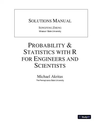
SOLUTIONSMANUALSONGFENGZHENGMissouri State UniversityPROBABILITY&STATISTICS WITHRFORENGINEERS ANDSCIENTISTSMichael AkritasThe Pennsylvania State University

Loading page image...

Contents1Basic Statistical Concepts11.2Populations and Samples . . . . . . . . . . . . . . . . . . . . . . . . . . .11.3Some Sampling Concepts . . . . . . . . . . . . . . . . . . . . . . . . . . .21.4Random Variables and Statistical Populations. . . . . . . . . . . . . . .31.5Basic Graphics for Data Visualization . . . . . . . . . . . . . . . . . . . .41.6Proportions, Averages, and Variances . . . . . . . . . . . . . . . . . . . .201.7Medians, Percentiles, and Boxplots. . . . . . . . . . . . . . . . . . . . .231.8Comparative Studies. . . . . . . . . . . . . . . . . . . . . . . . . . . . .242Introduction to Probability352.2Sample Spaces, Events, and Set Operations . . . . . . . . . . . . . . . . .352.3Experiments with Equally Likely Outcomes. . . . . . . . . . . . . . . .392.4Axioms and Properties of Probabilities. . . . . . . . . . . . . . . . . . .442.5Conditional Probability . . . . . . . . . . . . . . . . . . . . . . . . . . . .472.6Independent Events . . . . . . . . . . . . . . . . . . . . . . . . . . . . . .513Random Variables and Their Distributions533.2Describing a Probability Distribution. . . . . . . . . . . . . . . . . . . .533.3Parameters of Probability Distributions . . . . . . . . . . . . . . . . . . .593.4Models for Discrete Random Variables. . . . . . . . . . . . . . . . . . .633.5Models for Continuous Random Variables. . . . . . . . . . . . . . . . .684Jointly Distributed Random Variables774.2Describing Joint Probability Distributions. . . . . . . . . . . . . . . . .774.3Conditional Distributions . . . . . . . . . . . . . . . . . . . . . . . . . . .794.4Mean Value of Functions of Random Variables . . . . . . . . . . . . . . .874.5Quantifying Dependence. . . . . . . . . . . . . . . . . . . . . . . . . . .934.6Models for Joint Distributions . . . . . . . . . . . . . . . . . . . . . . . .975Some Approximation Results1035.2The LLN and the Consistency of Averages. . . . . . . . . . . . . . . . .1035.3Convolutions. . . . . . . . . . . . . . . . . . . . . . . . . . . . . . . . .1045.4The Central Limit Theorem. . . . . . . . . . . . . . . . . . . . . . . . .106

Loading page image...

CONTENTS6Fitting Models to Data1116.2Some Estimation Concepts . . . . . . . . . . . . . . . . . . . . . . . . . .1116.3Methods for Fitting Models to Data . . . . . . . . . . . . . . . . . . . . .1136.4Comparing Estimators: The MSE Criterion. . . . . . . . . . . . . . . .1197Confidence and Prediction Intervals1217.3Type of Confidence Intervals . . . . . . . . . . . . . . . . . . . . . . . . .1217.4The Issue of Precision. . . . . . . . . . . . . . . . . . . . . . . . . . . .1297.5Prediction Intervals . . . . . . . . . . . . . . . . . . . . . . . . . . . . . .1308Testing of Hypotheses1338.2Setting Up a Test Procedure . . . . . . . . . . . . . . . . . . . . . . . . .1338.3Types of Tests . . . . . . . . . . . . . . . . . . . . . . . . . . . . . . . . .1368.4Precision in Hypothesis Testing. . . . . . . . . . . . . . . . . . . . . . .1449Comparing Two Populations1479.2Two-Sample Tests and CIs for Means . . . . . . . . . . . . . . . . . . . .1479.3The Rank-Sum Test Procedure. . . . . . . . . . . . . . . . . . . . . . .1559.4Comparing Two Variances. . . . . . . . . . . . . . . . . . . . . . . . . .1589.5Paired Data . . . . . . . . . . . . . . . . . . . . . . . . . . . . . . . . . .15910 Comparingk >2Populations16310.2 Types ofk-Sample Tests. . . . . . . . . . . . . . . . . . . . . . . . . . .16310.3 Simultaneous CIs and Multiple Comparisons . . . . . . . . . . . . . . . .17310.4 Randomized Block Designs . . . . . . . . . . . . . . . . . . . . . . . . . .18111 Multifactor Experiments18711.2 Two-Factor Designs . . . . . . . . . . . . . . . . . . . . . . . . . . . . . .18711.3 Three-Factor Designs . . . . . . . . . . . . . . . . . . . . . . . . . . . . .19411.4 2rFactorial Experiments . . . . . . . . . . . . . . . . . . . . . . . . . . .19912 Polynomial and Multiple Regression20912.2 The Multiple Linear Regression Model. . . . . . . . . . . . . . . . . . .20912.3 Estimating, Testing, and Prediction . . . . . . . . . . . . . . . . . . . . .21212.4 Additional Topics . . . . . . . . . . . . . . . . . . . . . . . . . . . . . . .22113 Statistical Process Control23713.2 The¯XChart. . . . . . . . . . . . . . . . . . . . . . . . . . . . . . . . .23713.3 TheSandRCharts. . . . . . . . . . . . . . . . . . . . . . . . . . . . .24213.4 ThepandcCharts . . . . . . . . . . . . . . . . . . . . . . . . . . . . . .24613.5 CUSUM and EWMA Charts . . . . . . . . . . . . . . . . . . . . . . . . .249

Loading page image...

1Chapter 1Basic Statistical Concepts1.2Populations and Samples1.(a) The population consists of the customers who bought a car during the previousyear.(b) The population is not hypothetical.2.(a) There are three populations, one for each variety of corn. Each variety of cornthat has been and will be planted on all kinds of plots make up the population.(b) The characteristic of interest is the yield of each variety of corn at the time ofharvest.(c) There are three samples, one for each variety of corn. Each variety of corn thatwas planted on the 10 randomly selected plots make up the sample.3.(a) There are two populations, one for each shift.The cars that have been andwill be produced on each shift make up the population.(b) The populations are hypothetical.(c) The characteristic of interest is the number of nonconformances per car.4.(a) The population consists of the all domestic flights, past or future.(b) The sample consists of the 175 domestic flights.(c) The characteristic of interest is the air quality, quantified by the degree ofstaleness.5.(a) There are two populations, one for each teaching method.(b) The population consists of all students who took or will take a statistics coursefor engineering using one of each teaching methods.(c) The populations are hypothetical.(d) The samples consist of the students whose scores will be recorded at the endof the semester.

Loading page image...

2Chapter 1 Basic Statistical Concepts1.3Some Sampling Concepts1. The second choice provides a closer approximation to simple random sample.2.(a) It is not a simple random sample.(b) In (a), each member of the population does not have equal chance to beselected, thus it is not a simple random sample. Instead, the method describedin (a) is a stratified sampling.3.(a) The population includes all the drivers in the university town.(b) The student’s classmates do not constitute a simple random sample.(c) It is a convenient sample.(d) Young college students are not experienced drivers, thus they tend to use seatbelts less.Consequently, the sample in this problem will underestimate theproportion.4. We identify each person with a number from 1 to 70. Then we write each numberfrom 1 to 70 on separate, identical slips of paper, put all 70 slips of paper in a box,and mix them thoroughly. Finally, we select 15 slips from the box, one at a time,without replacement.The 15 selected numbers specify the desired sample of sizen= 15 from the 70 iPhones. The R command isy = sample(seq(1,70), size=15)A sample set is 52 8 14 48 62 6 70 35 18 20 3 41 50 27 40.5. We identify each pipe with a number from 1 to 90.Then we write each numberfrom 1 to 90 on separate, identical slips of paper, put all 90 slips of paper in a box,and mix them thoroughly. Finally, we select 5 slips from the box, one at a time,without replacement.The 5 selected numbers specify the desired sample of sizen= 5 from the 90 drain pipes. The R command isy = sample(seq(1,90), size=5),A sample set is7 38 65 71 57.6.(a) We identify each client with a number from 1 to 1000.Then we write eachnumber from 1 to 1000 on separate, identical slips of paper, put all 1000 slipsof paper in a box, and mix them thoroughly. Finally, we select 100 slips fromthe box, one at a time, without replacement. The 100 selected numbers specifythe desired sample of sizen= 100 from the 1000 clients.

Loading page image...

1.4 Random Variables and Statistical Populations3(b) Using stratified sampling:Get a simple random sample of size 80 from thesub-population of Caucasian-Americans, a simple random sample of size 15from the sub-population of African-Americans, and a simple random sampleof size 5 from the sub-population of Hispanic-Americans. Then combine thethree subsamples together.(c) The R command for part (a) isy = sample(seq(1,1000), size=100)and the R command for part (b) isy1 = sample(seq(1,800), size=80)y2 = sample(seq(801,950), size=15)y3 = sample(seq(951,1000), size=5)y = c(y1, y2, y3)7. One method is to take a simple random sample of sizenfrom the population ofNcustomers (of all dealerships of that car manufacturer) who bought a car theprevious year.The second method is to divide the population of the previous year’s customers intothree strata according to the type of car each customer bought and perform stratifiedsampling with proportional allocation of sample sizes. That is, ifN1,N2,N3denotethe sizes of the three strata, take simple random samples of approximate sizes (dueto round-off)n1=n(N1/N),n2=n(N2/N),n3=n(N3/N), respectively, fromeach of the three strata. Stratified sampling assures that the sample representationof the three strata equals their population representation.8. It is not a simple random sample because products from facility B have a smallerchance to be selected than products from facility A.9. No, because the method excludes samples consisting ofn1cars from the first shiftandn2= 9−n1from the second shift for any (n1, n2) different from (6,3).1.4Random Variables and Statistical Populations1.(a) The variable of interest is the number of scratches in each plate. The statisticalpopulation consists of 500 numbers, 190 zeros, 160 ones, and 150 twos.(b) The variable of interest is quantitative.(c) The variable of interest is univariate.2.(a) Statistical population: If there areNundergraduate students enrolled at PSU,the statistical population is a list of lengthNand thei-th element in the list isthe major of thei-th student. The variable of interest is qualitative. Anotherpossible variable: gender.

Loading page image...

4Chapter 1 Basic Statistical Concepts(b) Statistical population: If there areNrestaurants on campus, the statisticalpopulation consists of a list ofNnumbers, and thei-th element is the capacityof thei-th restaurant. The variable of interest is quantitative. Another possiblevariable: food type.(c) Statistical population: If there areNbooks in Penn State libraries, the sta-tistical population consists of a list ofNnumbers, and thei-th element is thecheck-out frequency of thei-th book in the library. The variable of interest isquantitative. Another possible variable: pages of the book.(d) Statistical population: If there areNsteel cylinders made in the given month,the population consists of a list ofNnumbers, and thei-th element is thediameter of thei-th steel cylinder made in the given month. The variable ofinterest is quantitative. Another possible variable: weight.3.(a) The variable of interest is univariate.(b) The variable of interest is quantitative.(c) IfNis the number cars of available for inspection, the statistical populationconsists ofNnumbers,{v1,· · ·, vN}, whereviis the total number of engineand transmission nonconformances of theith car.(d) If the number of nonconformances in the engine and transmission are recordedseparately for each car, the new variable would be bivariate.4.(a) The variable of interest is the degree of staleness. Statistical population consistsof a list of 175 numbers, and thei-th number is the degree of staleness of theair in thei-th domestic flight.(b) The variable of interest is quantitative.(c) The variable of interest is univariate.5.(a) The variable of interest is the type of car a customer bought and his/hersatisfaction level. Statistical population: If there areNcustomers who boughta new car in the previous year, the statistical population is a list ofNelements,and thei-th element is the car type thei-th customer bought along with his/hersatisfaction level, which is a number between 1 to 6.(b) The variable of interest is bivariate.(c) The variable of interest has two components. The first is qualitative and thesecond is quantitative.1.5Basic Graphics for Data Visualization1. The histogram produced by the commands is shown as following:

Loading page image...

1.5 Basic Graphics for Data Visualization5Histogram of StrStrDensity42444648500.000.100.20The stem and leaf plot is as following:The decimal point is at the|41|542|3943|144578844|12235745|144646|0024647|357748|3649|32. The histogram on the waiting time is as following

Loading page image...

6Chapter 1 Basic Statistical ConceptsHistogram of waitingwaitingFrequency40506070809010001020304050The corresponding stem and leaf plot is given below. It is clear that the shape ofthe stem and leaf plot is similar to that of the histogram.The decimal point is 1 digit(s) to the right of the|4|34|555666667777888999995|000001111112222233333334444444445|5555556666777888899999996|000000222233344446|5556678997|000011111233333334444447|5555555566666666677777777777788888888888888899999999998|0000000011111111111112222222222223333333333333344444444448|555555666666778888889999|000000123349|6The histogram with title and the colored smooth curve superimposed is shown as

Loading page image...

1.5 Basic Graphics for Data Visualization7Waiting times before Eruption the Old Faithful GeyserDensity4050607080901000.000.010.020.030.043. The scatterplot is shown below. From the scatter plot, it seems that if the waitingtime before eruption is longer, the duration is also longer.50607080901.52.02.53.03.54.04.55.0waitingeruptions4.(a) The scatterplot matrix is given below. From the figure, it seems that the lati-tude is a better predictor of the temperature because as the latitude changes,the temperature shows a clear pattern, while there is no pattern as the longi-tude changes.

Loading page image...

8Chapter 1 Basic Statistical ConceptsJanTemp253035404501030502530354045Lat0103050708090100120708090100120Long(b) The following figure gives the 3D scatter plot. The 3D scatter plot also showsthat the latitude is a better predictor for the temperature.253035404550010203040506070708090100110120130LatLongJanTemp

Loading page image...

1.5 Basic Graphics for Data Visualization95. The 3D scatterplot is shown below1015202530350100200300400500102030405060Neck.GChest.GWeight6. The scatterplot is shown below. From the scatterplot, it is clear that in general, ifthe speed is high, the breaking distance is larger.510152025020406080100120speeddist7. The required graph is given below:

Loading page image...

10Chapter 1 Basic Statistical Concepts204060801000100200300400500600SpeedStopDistCarsTrucks8. The resulting graph is given below. The figure shows that for SMaple and WOak,the growing speed in terms of the diameter of the tree is constant, while for ShHick-ory, when the tree gets older, it grows faster.406080100100150200250300diamageSMapleShHickoryWOak9.(a) The basic histogram with smooth curve superimposed:

Loading page image...

1.5 Basic Graphics for Data Visualization11Histogram of t1t1Density2829303132330.000.050.100.150.200.250.30(b) The stem and leaf plot for the reaction time of Robot 1 is given below. Thedecimal point is at the|28|429|013368830|0338831|023466932|4710. The produced basic scatter plot is given below. It seems that the surface conduc-tivity can be used for predicting sediment conductivity.

Loading page image...

12Chapter 1 Basic Statistical Concepts200300400500600700800400500600700800900XY11. The produced basic scatter plot is given below. It seems that the rainfall volumeis useful for predicting the runoff volume.2040608010012020406080100XY12. The produced scatterplot matrix is as following, and it seems that the variabletemperature is a better single predictor for the amount of electricity consumed.

Preview Mode

This document has 254 pages. Sign in to access the full document!

Report

Study Now!

Document Details

Related Documents

The Statistics of Inheritance

Estimation and Hypothesis Testing

Lab Activity 5 Sampling Distributions

Probability and Statistics Assignment

STAT 250-004 Data Analysis Assignment 4

Normal Distribution - Amount of Sleep

Correlation and Confidence Intervals

Two-Sample Hypothesis Tests

Hypothesis Testing � Comparing Two Groups

Inferential Statistics Week 2 Solution

Company

Explore

Study Tools