Solution Manual for Statistical Methods, 3rd Edition

Preview (16 of 215 Pages)

100%

Purchase to unlock

Loading page image...

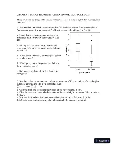
CHAPTER 1: SAMPLE PROBLEMS FOR HOMEWORK, CLASS OR EXAMSThese problems are designed to be done without access to a computer, but they may require acalculator.1. The boxplots shown below summarize data for vocabulary scores from two samples offirst-graders, some of whom attended Pre-K, and some of who did not (No Pre-K).a. Among Pre-K children, approximately whatproportion have vocabulary scores greater than41?b. Among no Pre-K children, approximatelywhat proportion have vocabulary scores between24 and 28?c. Which group apparently has the higher typicalvocabulary score?d. Which group shows the greater variability intheir vocabulary scores?e. Summarize the shape of the distribution foreach group.2. You jotted down some summary values for a data set of 15 observations of wave heights,in feet, at a monitoring site. Your notes state that:iy37 and2iy173.a. Give the mean and the standard deviation of the wave heights, in feet.b. Give the mean and the standard deviation of the wave heights, in meters. (Hint: a meter =3.3 feet).c. You also have written down that the median wave height, in feet, was 2 . Is thedistribution more likely negatively skewed, positively skewed, or symmetric?

Loading page image...

3. Volunteers in a psychology experiment watch a video re-enactment of a crime. After adelay, they answer questions about the scene. The researcher records both the length of thedelay (in hours) and the number of questions the volunteer answered correctly. A graphicaldisplay of the data is shown below.Write a sentence, in simple language,that summarizes the relationshipbetween the two variables.4. A school is concerned that the playground area may have contaminated soil left from atime when a creosote plant was nearby. The school can not afford to test all the soil on theplayground, so a statistician divides a map of the playground into 1000 equally sizedrectangles. A random number generator is used to select 30 rectangles. A soil specimen istaken from each selected rectangle.a. Identify the population, the sampling frame, and the sample.b. Is this study observational or a designed experiment?c. For each variable, say whether its scale is nominal, ordinal, interval or ratio. Identify onetype of graph that can be used to summarize the data.Contamination level (none, trace, moderate, high)Creosote concentration, in parts per billionUsage (general play, organized sports, drainage structure, etc.)5. Barometric pressures in tropical cyclones are very negatively (left) skewed. You wrotedown 1005 and 985 as the mean and median, but forgot to label which was which. Label thevalues properly.

Loading page image...

6. The two histograms below summarize total cholesterol levels for large samples of elderlymen and women. Write a short paragraph comparing the two groups. Be sure to contrast thetypical values, variability and shape of the distributions.051015202530PercentF112. 5137. 5162. 5187. 5212. 5237. 5262. 5287. 5312. 5337. 5362. 5387. 5051015202530PercentMchol7.The frequency table below summarizes the results for mercury concentrations in asample of Florida lakes. Display the relative frequencies using an appropriate graph.Mercury ConcentrationNumber of casesTrace (very low)11Low27Borderline8Dangerous3

Loading page image...

8. The data below shows electricity costs in cents per KWH for a sample of 14 utilitycompanies. The data has already been sorted, reading across each row.12.412.813.113.613.813.914.014.214.214.414.614.815.015.3a. Calculate the first quartile, median, and third quartile.b. Calculate the range and the interquartile range.c. Identify the outliers, if there are any. Show your computations.d. Construct the boxplot for this data, and comment on the shape of the distribution.9. The boxplots show NOx emissions from your power plant (expressed as pounds per MWhof electricity generated), using two different settings for the air intakes. Compare theemissions, being sure to address the typical values, variability, shape and/or other specialfeatures. If your goal is to lower typical NOx emissions, which setting should you select? Ifyour goal is to avoid any extremely high values, which setting should you select?settingHIGHLOWNOx8.006.004.002.0010. a. In a data set with a sample mean of 10 and a standard deviation of 2, you note that78% of observations fall in the interval (6, 14). Is this distribution approximately bell-shaped? Why or why not?b. In a data set with a sample mean of 10 and a standard deiation of 2, you wrote down thepercent of the observations that fall in the interval (6, 14). Later, you find your writing is hardto read, but the number is either 63% or 83%. Which must it be and why?SOLUTIONS1. a. 25%b. 25%c. The pre-K group apparently has higher typical values.d. The No pre-K group shows slightly higher variability.e. Scores in the pre-K group are nearly symmetrically distributed, but in the No pre-K groupthey are positively (or right) skewed.

Loading page image...

2. a. mean = 2.47, SD = 2.42b. this is a simple change of scale. Mean = 2.47/3.3 = 0.75, SD = 2.42/3.3 = 0.73c. Since the mean is substantially greater than the median, the distribution is most likelyright, or positively, skewed. Alternately, one might see that the size of the SD compared tothe mean, combined with the fact that there are no negative wave heights, implies a positiveskew.3. As the time delay increases, the number of questions answered correctly tends to decrease.4. a. The population is all soil in the playground, or alternatively all 1000 rectangles of soil.The sampling frame is the list of the 1000 rectangles. The sample is the 30 rectanglesselected for study.b. Observationalc. Contamination level is ordinal, use bar chart or pie chart;Creosote concentration is ratio, use a histogram, boxplot or stem-and-leaf plot.Usage is nominal, use a bar chart or pie chart.5. Since the data is very left skewed, the mean must be less than the median. Mean = 985,median = 1005.6. Typical values for the females are slightly higher than those for the men. Females showslightly higher variability, though the difference in variability is not large. Both distributionsshow some right skew, but the skew is stronger in the males.7. The bar chart is shown below. Pie charts are possible, but are harder to draw and harder tocompare when there is more than one sample.8. a. median = (14.0+14.2)/2 = 14.1Using the algorithm described in the text, Q1 = 13.35 and Q3 = 14.5However, a variety of algorithms exist, on the TI83/84 calculators, Q1 = 13.6 and Q3 = 14.6.b. Range = 2.9. IQR = 1.15 using algorithm for quartiles given in book, but IQR = 1 usingTI83/84.c. Using algorithm for quartiles given in book, lower fence = 11.625 and upper fence =16.225. There are no outliers.d. will depend slightly on algorithm for outliers. Nearly symmetric, but some students willnot a slight negative skew.9. The typical NOx values are lower at the High air intake setting, as shown by the lowermedian. However, the NOx values are more variable at the high air intake setting, andsomewhat right-skewed. At the low intake setting, the values are more symmetric and lessvariable. Hence, to lower the typical NOx values one should choose the high air intakesetting, but to avoid extremely high values, one needs to use the low air intake setting.

Loading page image...

10. a. This distribution cannot be approximately bell-shaped because if it were thepercentage in this interval (mean ± 2 std.dev) would be close to 95%.b. It must be 83%, because this interval (mean ± 2 std. dev) must include at least 75% of theobservations, using Tchebysheff’s Theorem.

Loading page image...

Chapter 1 – Page 1CHAPTER 1EXERCISE 1a)Mean = 17.00, SD = 5.53, median = 17.00,Range = 22,IQR = 20 – 13 = 7.b)See boxplot.c)A typical value for X is 17 which is both the mean and themedian. About half the values are between 13 and 20. The boxplotshows that the upper tail is slightly longer, but difference is smalland mean and median are equal. This distribution is roughlysymmetric.

Loading page image...

Chapter 1 – Page 2EXERCISE 2VariableMeanMedianVarianceStandardDeviationShapeWATER7.1251.500452.86421.28extremely positivelyskewedVEG1.1200.004.3272.080extremely positivelyskewedFOWL75.63511.542197.33205.420extremely positivelyskewedWATERStem Leaf#Boxplot14 91*131211109876543 132*21 05667500 0000000000000111111111111222222222234555677944+--+--+----+----+----+----+----+----+----+----+----Multiply Stem.Leaf by 10**+1VEGStem Leaf#Boxplot9 01*88 01*77 01*6655 21044 01|3|3 01|2 81|2 000025|1 582+-----+1 00024|+|0 582||0 0000000000000000000000000000000232*-----*----+----+----+----+----+----+--

Loading page image...

Chapter 1 – Page 3FOWLStem Leaf#Boxplot14 11*131211109876543 61*2 124301 227888600 0000000000000000000000111111222222333567841+--+--+----+----+----+----+----+----+----+----+-Multiply Stem.Leaf by 10**+2b)Frequency distribution for FOWLFowlFrequencyMidpointapproximatemean=5500/520≤x<1004150.0=105.8100≤x<2006150.0200≤x<3003250.0approximatevariance=50746300≤x<4001350.01400≤x<150011450.0c)ScatterplotsAside from the single point with extraordinary number of waterfowl, there is little relationship.fowl0100200300400500600700800900100011001200130014001500veg0123456789

Loading page image...

Chapter 1 – Page 4EXERCISE 3a)INDEX:mean = -0.149median = -0.155variance = 1.771IQR = 1.59 (show stem and leaf,histogram, or boxplot as part ofanswer)FUTURE:mean = -0.208median = -0.3variance = 0.601IQR = 0.81 (show stem and leaf,histogram, or boxplot as part ofanswer)b)The Scatter plot is shown below. There is a clear trend for positive changes in the FUTURE contractvalue to be associated with positive changes in the NYSE INDEX. Yes, FUTURE can be used to helppredict changes in the NYSE index.index-4-3-2-10123future-3-2-1012

Loading page image...

Chapter 1 – Page 5EXERCISE 4Y1Stem Leaf#Boxplot8 142|7 31|6 12378897+-----+5 3383*-----*4 0253|+|3 1123+-----+2 4783|1 6683|----+----+----+----+Y2Stem Leaf#Boxplot6 56794|6 41|5 7893+-----+5 222||4 6783*--+--*4 00244||3 5593+-----+3 123335|----+----+----+----+Y3Stem Leaf#Boxplot9 41|8 01|7|6 7773|5 4443+-----+4 0003||3|+|2 77777777*-----*1 3333336+-----+0 01|----+----+----+----+

Loading page image...

Chapter 1 – Page 6Y4Stem Leaf#Boxplot7 41|6|5 01|4 5783|3 992+-----+2 1233576*--+--*1 014685||0 11136997+-----+----+----+----+----+Y1 is slightly negatively (or left) skewed; Y2 is nearly symmetrically distributed, though without a welldefined peak; Y3 is positively (or right) skewed; Y4 is extremely positively skewed.comparison to empirical rule, actual percentage of observations in intervalmeanStd devShape±1 SD (expect68%)±2 SD (expect95%)±3 SD(expect all)Y14.8402.107slight left skew68%100%100%Y24.7481.262near symm.60%100%100%Y33.6962.434right skew76%96%100%Y42.3281.888extreme rightskew64%96%100%The empirical rule works reasonably well even for the skewed distributions.

Loading page image...

Chapter 1 – Page 7EXERCISE 5a)DAYS:Mean= 15.854median= 17, variance= 24.324TEMP:Mean= 39.348median= 40 variance= 11.152b)Scatterplot:days0102030temp303132333435363738394041424344454647

Loading page image...

Chapter 1 – Page 8From the scatterplot, there appears to be no definitive relationship between the average temperature andthe number of rainy January days.EXERCISE 6a)The distribution of EXPEND is extremely right skewed with a mean ($1816M) that is much greaterthan the median ($1169M), so the best measure of location is the median and the best measure ofdispersion is the IQR ($1938M). There are three outlier states with California being an extreme outlier at$15348M.b)Per Capita expenditures are also right skewed, but slightly less so than expenditures. The median is$0.269k ($2,690) and the IQR is $0.139k.c)For Per Capita expenditures, there is one state that is an extreme outlier (Alaska) and another that is amoderate outlier (Delaware). Both these are states with small populations, which may mean that there area lot of fixed costs in the systems.EXERCISE 7 Scatter of DFOOT vs. HCRN:Scatter ofdfoot23456hcrn123456789

Loading page image...

Chapter 1 – Page 9dfoot vs. ht:Scatter of HCRN vs. HT:Thestrongest relationship exists between DFOOT, the diameter of the tree at one foot above ground level andHT, the total height of the tree. (notice from the scatter plot that it is closest to a linear relationship) Onewould expect that as the base of the tree increases in diameter the tree would increase in height as well.dfoot23456ht20212223242526272829303132hcrn123456789ht20212223242526272829303132

Preview Mode

This document has 215 pages. Sign in to access the full document!

Report

Study Now!

Document Details

Related Documents

The Statistics of Inheritance

Estimation and Hypothesis Testing

Lab Activity 5 Sampling Distributions

Probability and Statistics Assignment

STAT 250-004 Data Analysis Assignment 4

Normal Distribution - Amount of Sleep

Correlation and Confidence Intervals

Two-Sample Hypothesis Tests

Hypothesis Testing � Comparing Two Groups

Inferential Statistics Week 2 Solution

Company

Explore

Study Tools