Page 1

Loading page image...
Page 2

Loading page image...
Page 3
Loading page image...
Page 4
Loading page image...
Page 5
Loading page image...
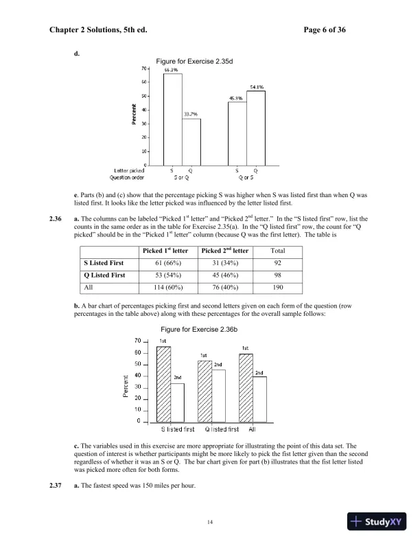
Page 6
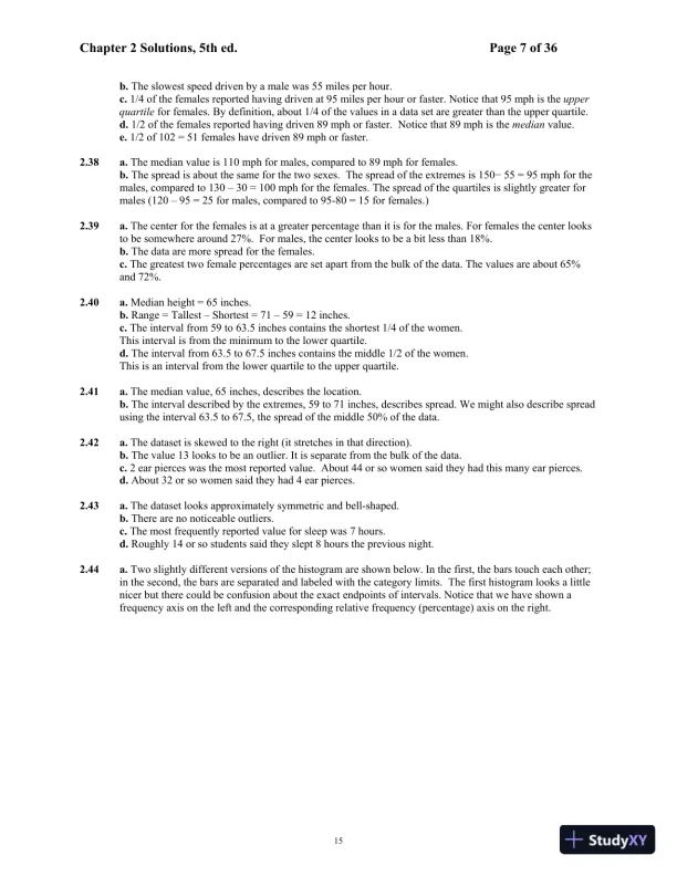
Loading page image...
Page 7
Loading page image...
Page 8
Loading page image...
Page 9
Loading page image...
Page 10
Loading page image...
Page 11
Loading page image...
Page 12
Loading page image...
Page 13
Loading page image...
Page 14
Loading page image...
Page 15
Loading page image...
Page 16
Loading page image...