Solution Manual for Using Econometrics: A Practical Guide, 7th Edition

Preview (5 of 16 Pages)

100%

Purchase to unlock

Loading page image...

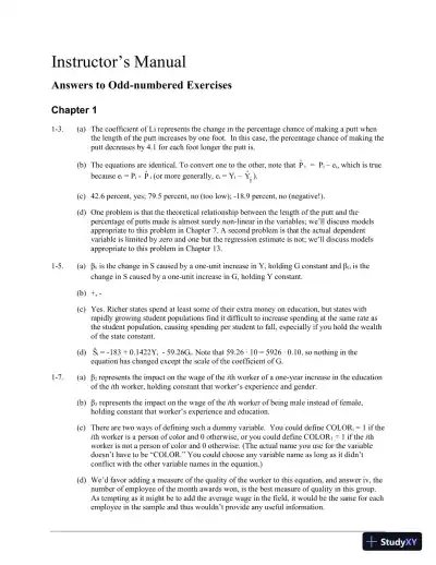
Instructor’s ManualAnswers to Odd-numbered ExercisesChapter11-3.(a)Thecoefficientof Li represents the change in the percentage chance of making a putt whenthe length of the putt increases by one foot. In this case, the percentage chance of making theputt decreases by 4.1 for each foot longer the putt is.(b)The equations are identical. To convert one to the other, note thatˆPi= Pi–ei, which is truebecause ei= Pi-ˆPi(or more generally, ei= Yi–ˆYi).(c)42.6 percent, yes; 79.5 percent, no (toolow);-18.9 percent, no (negative!).(d)One problem is that the theoretical relationship between the length of the putt and thepercentage of putts made is almost surely non-linear in the variables; we’ll discuss modelsappropriate to this problem in Chapter 7. A second problem is that the actual dependentvariable is limited by zero and one but the regression estimate is not; we’ll discuss modelsappropriate to this problem in Chapter 13.1-5.(a)βʏis the change in S caused by a one-unit increase in Y, holding G constant andβGis thechange in S caused by a one-unit increase in G, holding Y constant.(b)+,-(c)Yes. Richer states spend at least some of their extra money on education, but states withrapidly growing student populations find it difficult to increase spending at the same rate asthe student population, causing spending per student to fall, especially if you hold the wealthof the state constant.(d)Ŝi=-183 + 0.1422Yi-59.26Gi. Note that 59.26 ∙ 10 = 5926 ∙ 0.10, so nothing in theequation has changed except the scale of the coefficient of G.1-7.(a)β2represents the impact on the wage of theith worker of a one-year increase in the educationof theith worker, holding constant that worker’s experience and gender.(b)β3represents the impact on the wage of theith worker of being male instead of female,holding constant that worker’s experience and education.(c)There are two ways of defining such a dummy variable. You could define COLORi= 1 if theith worker is a person of color and 0 otherwise, or you could define COLOR1= 1 if theithworker is not a person of color and 0 otherwise. (The actual name you use for the variabledoesn’t have to be “COLOR.” You could choose any variable name as long as it didn’tconflict with the other variable names in the equation.)(d)We’d favor adding a measure of the quality of the worker to this equation, and answer iv, thenumber of employee of the month awards won, is the best measure of quality in this group.As tempting as it might be to add the average wage in the field, itwould be the same for eachemployee in the sample and thus wouldn’t provide any useful information.

Loading page image...

2Studenmund•Using Econometrics,Seventh EditionChapter22-3.(a)The squares are “least” in the sense that they are being minimized.(b)If R2=0, then RSS=TSS, and ESS=0. If R2is calculated as ESS/TSS, then it cannot benegative. If R2is calculated as 1–RSS/TSS, however, then it can be negative if RSS > TSS,which can happen ifˆYis aworsepredictor of Y thanY(possible only with a non-OLSestimator or if the constant term is omitted).(c)positive.(d)We prefer Model T because it has estimated signs that meet expectations and also because itincludes an important variable thatModel A omits. A higher R2does notautomaticallymeanthat an equation is preferred.2-5.(a)Even though the fit in Equation A is better, most researchers would prefer equation Bbecause the signs of the estimated coefficients are as would be expected. In addition, X4is atheoretically sound variable for a campus track, while X3seems poorly specified because anespecially hotorcold day would discourage fitness runners.(b)The coefficient of an independent variable tells us the impact of a one-unit increase in thatvariable on the dependent variable holding constant the other explanatory variables in theequation. If we change the other variables in the equation, we’re holding different variablesconstant, and so theˆhas a different meaning.2-7.(a)Yes.We’d expect bigger colleges to get more applicants, and we’d expect colleges that usedthe common application to attract more applicants. It might seem at first that the rank of acollege ought to have a positive coefficient, but the variable is defined as 1 = best, so we’dexpect a negative coefficient for RANK.(b)The meaning of the coefficient of SIZE is that for every increase of one in the size of thestudent body, we’d expect a college to generate 2.15 more applications, holding RANK andCOMMONAP constant. The meaning of the coefficient of RANK is that every one-rankimprovement in a college’s USNews ranking should generate 32.1 more applications,holding SIZE and COMMONAP constant. These results do not allow us to conclude that acollege’s ranking is 15 times more important than the size of that college because the units ofthe variables SIZE and RANK are quite different in magnitude. On a more philosophicallevel, it’s risky to draw any general conclusions at all from one regression estimated on asample of 49 colleges.(c)The meaning of the coefficient of COMMONAP is that a college that switches to using thecommon application can expect to generate 1222 more applications, holding constant RANKand SIZE. However, this result does not prove that a given college would increaseapplications by 1222 by switching to the common application. Why not? First, we don’ttrust this result because there may well be an omitted relevant variable (or two) and becauseall but three of the colleges in the sample use the common application. Second, in general,econometric results are evidence that can be used to support an argument, but in and ofthemselves they don’t come close to “proving” anything.(e)If you drop COMMONAP from the equation,2Rfalls. This is evidence (but not proof) thatCOMMONAP belongs in the equation.

Loading page image...

An Additional Interactive Regression Learning Exercise3Chapter33-3.(a)A male professor in this sample earns $817 more than a female professor, holding constantthe otherindependent variables in the equation.(b)Most students will expect a negative coefficient, so they will call this an unexpected sign.Most professors and administrators will expect a positive sign because of the growingcompetition among colleges for African-American professors, so they will call this anexpected sign. A key point here is not to change expectations based solely on this result.(c)R is not a dummy variable because it takes on more than two values. For each additional yearin rank, the ith professor’s salary will rise by $406, holding constant the other independentvariables in the equation.(d)Yes. The coefficient is large and, as we’ll learn in Chapter 5, statistically significantlygreater than zero. (In addition, it’s quite robust.)(e)There’s no measure of the quality of the professor in the equation as it stands, so goodsuggestions might the number of articles published by theith professor or the averageteaching evaluation (on a standard scale) of theith professor.3-5.(a)A male student’s GRE subject score in Economics is likely to be 39.7 points higher than afemale’s, holding constant their GPA and SATs.(b)This result is evidence of, but not proof of, bias. If we were sure that we had the bestpossible specification (the topic of Chapter 6) and if this result turned out to be statisticallysignificant (the topic of Chapter 5), and if we were able to reproduce this result in othersamples, we’d be much closer to a “proof.” Even then, there still would be a possibility thatsome factor other than bias was the cause of these results.(c)Possible variables include the number of upper division economics courses taken, the numberof mathematics classes taken, and dummy variables measuring whether the student had takeneconometrics or international economics (two fields frequently covered in the test). It’s vitalthat any suggested variable becross-sectional by student.(d)The equation would becomeiGRE= 212.1–39.7Gi+ 78.9GPAi+ 0.203SATMi+0.110SATVi..3-7.(a)The best way to handle three discrete conditions is to specify two dummy variables. Forexample, one dummy variable could =1 if the iPod is new (and 0 otherwise) and the otherdummy variable could =1 if the iPod is used but unblemished (and 0 otherwise).The omittedcondition, that the iPod is used and scratched, would be represented by both dummyvariables equaling zero.(b)Positive, negative, positive(c)In theory, the narrower the time spread of theobservations, the better the sample, but threeweeks probably is a short enough time period to ensure that the observations are from thesame population. If the three weeks included a major shock to the iPod market, however,then the friend would be right, and the sample should be split into “before the shock” and“after the shock” subsamples.(d)Yes, they match with the answer to part b.

Loading page image...

4Studenmund•Using Econometrics,Seventh Edition(e)2Ris missing!(f)2Ris .431.Chapter44-3.Pair“c”clearly violates Assumption VI, and pair“a”probably violates it for most samples.4-5.(a)Yes, Yes. In particular, there’s no measure of prices in the equation.(b)Yes(c)Yes, Very unlikely(d)No(e)No(f)No(g)Thenightclub should hire a dancerbecause the estimated coefficient is higher.Chapter55-3.(a)H0:β10, HA:β1>0(b)H0:β1≥ 0, HA:β1<0; H0:β2≤ 0, HA:β2>0;H0:β3≤ 0, HA:β3>0 (The hypothesis for β3assumes that it is never too hot to go jogging.)(c)H0:β10, HA:β1>0; H0:β2≤ 0, HA:β2>0;H0:β3≥ 0, HA:β3<0; (The hypothesis for β3assumes you’re not breaking the speed limit.)(d)H0:βG= 0; HA:βG0 (G for grunt.)5-5.(a)t2= (200–160)/25.0 = 1.6; tc= 2.052; therefore cannot reject H0. (Notice the violation of theprinciple that the nullhypothesiscontains that which we do not expect.)(b)t3= 2.37; tc= 2.756; therefore cannot reject the null hypothesis.(c)t2= 5.6; tc= 2.447; therefore reject H0if it is formulated as in the exercise, but this poses aproblem because the original hypothesized sign of the coefficient was negative. Thus, thealternative hypothesis ought to have been stated: HA:β2< 0, andH0cannot be rejectedbecause the sign of t2doesn’t agree withthe sign in thealternative hypothesis.5-7.(a)For both, H0:β ≤ 0 and HA: β > 0. For WIN, we cannot rejectH0,even though the sign agreeswith the sign implied by HA, because |+1.00| < 1.697, the 5 percent one-sided criticalt-valuefor 30 degrees of freedom. For FREE, we can rejectH0at the 5 percent level of significancebecause |2.00|> 1.697 and because 2.00 has the sign implied by HA.

Preview Mode

This document has 16 pages. Sign in to access the full document!

Report

Study Now!

Document Details

Related Documents

Analysis of McDonald

The Effect of Exercise on Clothespin Squeezing

Analyzing Coca-Cola's Demand, Supply and Market St

Emerging Economies and Globalization

Principles of Managerial Economics

Emerging Economies and Globalization

United States Fiscal Policy

Economic Policy Recommendation

Assignment 2: Market Forms

Should the U.S. convert to a Zero Personal Income Tax

Company

Explore

Study Tools