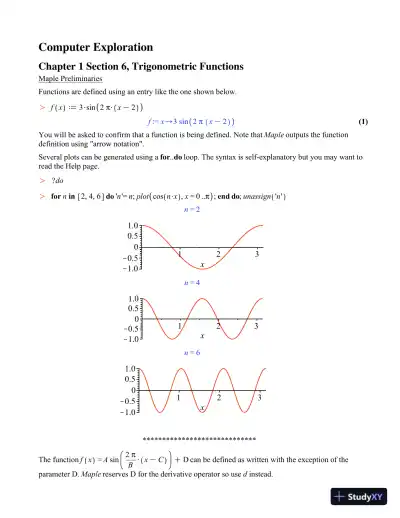
O (1) O O Computer Exploration Chapter 1 Section 6, Trigonometric Functions Maple Preliminaries Functions are defined using an entry like the one shown below. f x d 3 $ sin 2 ! $ x K 2 f := x / 3 sin 2 ! x K 2 You will be asked to confirm that a function is being defined. Note that Maple outputs the function definition using "arrow notation". Several plots can be generated using a for .. do loop. The syntax is self-explanatory but you may want to read the Help page. ? do for n in 2, 4, 6 do ' n '= n ; plot cos n $ x , x = 0 .. ! ; end do ; unassign ' n ' n = 2 x 1 2 3 K 1.0 K 0.5 0 0.5 1.0 n = 4 x 1 2 3 K 1.0 K 0.5 0 0.5 1.0 n = 6 x 1 2 3 K 1.0 K 0.5 0 0.5 1.0 ***************************** The function f x = A sin 2 ! B $ x K C C D can be defined as written with the exception of the parameter D. Maple reserves D for the derivative operator so use d instead. (2) O O O (3) f x d A sin 2 ! B $ x K C C d f := x / A sin 2 ! x K C B C d Vary one parameter at a time by assigning values to the other three. Values can be assigned in one entry as shown below. A , C , d d 3, 0, 0 : ' f x ' = f x f x = 3 sin 2 ! x B A for .. do loop can be used to make the plots. Adjust the plot windows so they are the same size. To do this click on the plot and use the mouse to drag the handles on edges of the box that enclose the plot. for B in 1, 3, 6 do ' B '= B ; plot f x , x = K 4 ! ..4 ! , K 4 ..4 ; end do ; unassign ' B ' B = 1 x K 10 K 5 5 10 K 4 K 1 1 4 B = 3 x K 10 K 5 5 10 K 4 K 1 1 4 B = 6 x K 10 K 5 5 10 K 4 K 1 1 4 !"# ! ! ! !"#$%ter)*+$,"r-t."n !0-$ter)2)2ect."n)15)6-tes)"8)!0-n9e !"#$%&'()*&++,#*(-*.#/(-#+)0)/)1$#2&+3-#"4#/(-#431*/)"1 ! " d " 5 K 6 " 5 C 7 K 8 ! 9: " / " 5 K 6 " 5 C 7 K 8 &;# " / <=#>-$)1#?)/(#&#'+"/#4"%# " #2&+3-;#1-&%#<=#+-//)1$# #$%&' #*("";-#/(-#2-%/)*&+#%&1$-@#A"B#/(-#&B-;#/"# 4"*3;#&//-1/)"1#/"#/(-#>"31C;#"4#/(-#'+"/@ %&() ! " =# " : 5 @@8=# $"'* : +("', " 5@D 5@E <@D <@E 8@D 7@F G@D G@F H/#&''-&%;#/(&/#/(-#+)0)/)1$#2&+3-#);#G@#I-/#*+";-%=#&CC)1$#&#("%J"1/&+#+)1-#&/# - : G#&1C#&#2-%/)*&+#+)1-#&/# " : <@ %&() ! " = G= <= - = - : ! 5@E @@ ! <@E =# " : 5@E @@<@E= $"'* : +("', = ########################### .(&(/ : /', = +&$.0 = +&$.0 " 5@F 5@G <@D <@5 <@8 7@7 7@6 G@K G@< L"/-@#!(-#2-%/)*&+#+)1-#?&;#C%&?1#&;#&#'&%&0-/%)J-C#*3%2-#?)/(#/(-#-1/%, <= - = - : ! 5@E @@ ! <@E @ !"#0&.-#;3%-=#$-/#-2-1#*+";-%@ (3) O O O (1) (2) O O Computer Exploration Chapter 2 Section 3, The Precise Definition of a Limit Maple Preliminaries To evaluate a limit type limit then press [esc]-[enter] to enter a limit template. Tab from position to position. lim x / a f x f a If no information is given, then Maple assumes that the function f is continuous at a . ***************************** Using a plot of the function f x d 3 x 2 K 7 x C 1 x C 5 x K 1 f := x / 3 x 2 K 7 x C 1 x C 5 x K 1 near to x 0 = 1 our guess is that the limiting value of f is L = K 5. plot f x , x = 0 ..2 x 0.0 0.5 1.0 1.5 2.0 K 5.1 K 4.9 K 4.7 K 4.5 K 4.3 The following limit calculation confirms that this is the case. lim x / 1 f x K 5 Based upon the picture above we can make the following preliminary plot. Note that a horizontal line at y = 5 has been added to the plot, and we have boxed the axes. plot f x , K 5 , x = 0.5 ..1.5, y = K 5.2 .. K 4.8, axes = boxed O O x 0.6 0.8 1.0 1.2 1.4 y K 5.2 K 5.1 K 5.0 K 4.9 K 4.8 It appears that ! = 0.3 will do the job for e = 0.2. See the following picture. plot f x , K 5 , x = 1 K 0.3 ..1 C 0.3, y = K 5 K 0.2 .. K 5 C 0.2, axes = boxed x 0.8 0.9 1.0 1.1 1.2 1.3 y K 5.2 K 5.1 K 5.0 K 4.9 K 4.8 (1) (3) ! ! ! ! ! ! (2) ! ! ! ! ! ! Computer Exploration Chapter 2 Section 7, Tangents and Derivatives Problem 45. Begin with the definition of the function f and the difference quotient function q . f x d x 3 C 2 x : q h d f 0 C h K f 0 h : Here is a plot of f . plot f x , x = K 1 2 ..3 x 0 1 2 3 10 20 30 Let m 0 denote the limit of the difference quotient as h / 0. m 0 d lim h / 0 q h m 0 := 2 The tangent line function is defined next. T x d m 0 $ x K 0 C f 0 T := x / m 0 x C f 0 And the next entry defines the secant line at 0 as a function of x and h. S x , h d q h $ x K 0 C f 0 S := x , h / q h x C f 0 The plots follow. The tangent line is blue and the secant lines are green. plot f x , T x , S x , 1 , S x , 2 , S x , 3 , x = K 1 2 ..3, color = red , blue , green $3 x 0 1 2 3 10 20 30 (3) (1) O (4) (2) O O O O Computer Exploration Chapter 3 Section 1, The Derivative as a Function Maple Preliminaries The unapply procedure An expression obtained as output can be converted into a function using the procedure called unapply . Here is an example. First enter an algebraic expression and use simplify to simplify it. x 3 K 1 x 2 K 1 ; simplify % x 3 K 1 x 2 K 1 x 2 C x C 1 x C 1 Now make the simplified expression into a function as follows. g d unapply (1) , x g := x / x 2 C x C 1 x C 1 Labels The label for output (1) was entered by pressing [Control]-L ( [Command]-L on a Macintosh), entering the number 1 in the ensuing dialogue, and pressing the [enter] key. The repetition operator The repetition operator : $ , is useful for making sequences. It works like this. F x $ x = 0 ..4 F 0 , F 1 , F 2 , F 3 , F 4 Here is a nice example. cos k ! 6 $ k = 0 ..6 1, 1 2 3 , 1 2 , 0, K 1 2 , K 1 2 3 , K 1 The Matrix procedure Tabulated data can be displayed using the Matrix procedure. For example, some values of the function g can be displayed like this. Note the use of the repetition operator. Matrix x , 0.2 k $ k = K 2 ..2 , '' g x '', g 0.2 k $ k = K 2 ..2 : evalf 4 % O O O (5) (6) O (8) (7) O x K .4 K .2 0. 0.2 0.4 g x 1.267 1.050 1.000 1.033 1.114 There are two single quotes around g x to postpone evaluation, twice. ******************** We explore the following function near x 0 = K 1. f x d x K 1 3 x 2 C 1 f := x / x K 1 3 x 2 C 1 Its graph reveals its global behavior. plot f x , x = K 3 ..3 x K 3 K 2 K 1 1 2 3 K 1.0 K 0.6 K 0.2 The definition of the difference quotient at a general x value follows. The quotient is simplified first. q d unapply simplify f x C h K f x h , x , h q := x , h / K 3 x 2 K 1 C 3 x h K 6 x K 3 h 3 x 2 C 6 x h C 3 h 2 C 1 3 x 2 C 1 Here is its limit as h / 0 . It defines a function of x that we call m . m d unapply lim h / 0 q x , h , x m := x / K 3 x 2 K 1 K 6 x 3 x 2 C 1 2 The function and its tangent line at the point K 1, f K 1 is plotted below. The tangent line is defined first as a parametrized curve named TanLine . TanLine d t , f K 1 C m K 1 $ t C 1 , t = K 1.5 .. K 0.5 : plot f x , TanLine , x = K 3 ..3, color = red , blue , thickness = 1, 2 O (9) O x K 3 K 2 K 1 1 2 3 K 1.0 K 0.6 K 0.2 The following matrix displays values of the function m at evenly spaced points to the left and right of x 0 = K 1. Matrix x , K 1 C 0.5 k $ k = K 2 ..2 , '' m x '', m K 1 C 0.5 k $ k = K 2 ..2 : evalf 4 % x K 2.0 K 1.5 K 1. K .5 0. m x K .1361 K .2456 K .5000 K .8980 1.000 A plot of f and m on the same axes can be used to help understand the relationship between these two functions. plot f x , m x , x = K 3 ..3 x K 3 K 2 K 1 0 1 2 3 K 1.0 K 0.5 0.5 1.0 1.5 ! ! !"# !$# ! ! !%# !&# ! ! ! ! ! ! !'# ! ! !(# ! ! !)# !"#$%&'()*+$,"(-&."/ !0-$&'()1)2'3&."/)45)60')!0-./)7%,')-/8)9-(-#'&(.3)*:%-&."/; 6(.<"/"#'&(.3)9",=/"#.-,; Maple&'relimi+arie, !"#$%#&'()*'(#$+,-.*'/- -avi+/&0efi+e0&a&f2+3tio+&2,i+/&f2+3tio+&+otatio+&t6e&2,2al&prime&+otatio+&3a+&7e&2,e0&to&o7tai+&it,& 0erivative&f2+3tio+8 f x d x 9 ! x f :; x ! x 9 ! x f < x 9& x ! = 0&'1#$-/*)*'/-$/-$)$()&')23# >f&a&prime&i,&applie0&to&varia7le?&t6e+&Maple&a,,2me,&t6at&t6e&varia7le&i,&a&f2+3tio+&of& x &a+0&t6e&prime& mea+,&0iffere+tiatio+&@it6&re,pe3t&to&t6e& x &varia7le8 y <&?& $ < 0 0 x & y x ? 0 0 x & $ x Aote&t6e&follo@i+/8 x <?& x 9 " x < =? 9& x " = B6e&C6ai+&D2le&@ill&7e&applie0&a,&+ee0e08&Eee&7elo@8 w x " w x 9 & " &,i+ w x < 0 0 x & w x " 9& w x & 0 0 x & w x " 3o, w x & 0 0 x & w x !"#$)%%$4&/.#%,&# F,e&t6e& add &pro3e02re&to&a00&a&fi+ite&+2m7er&of&term,8&B6ere&are&t@o&@aG,&to&make&it&@ork8 add & ( 9 ?& ( ; = 88I JK add &,i+ ( ?& ( ; =? 9? L? M? N? O ,i+ = " ,i+ 9 " ,i+ L " ,i+ M " ,i+ N " ,i+ O PPPPPPPPPPPPPPPPPPPP B6e&tri/o+ometri3&polG+omial&for&t6e&,a@toot6&f2+3tio+&i,&0i,plaGe0&7elo@8&B6e&3oeffi3ie+t,&@ere& o7tai+e0&i+&a&3al32latio+&t6at&i,&6i00e+&from&vie@8& ! ! (9) ! ! ! ! ! ! ($) ! ! ! d "#$%%&' $ " ! $(( $ # " #$% & # ) ' # ( )' *' +' , ' ) - . ! ) .( ! ) ! ) ( "/,0+*10& # "/2*22)10 #$% & ) # "/",",*++* #$% 2 ) # "/"&+323,1 #$% )" ) # "/")&11&&3 #$% )3 ) 456 789#:;$9 :5<: ! <==>$?;@<:6% #<9 A6 B67;96B $9 :56 ;9:6>C<D # "/+ ! " ) " "/+ ! 8%;9E :56 %*+,+-*.+ =>$#6B8>6/ F66 :56 G6D= =<E6 7$> %*+,+-*.+ / / 0 d %*+,+-*.+ 0 " "/+ ! ' 0 / -( 0 ! %*+,+-*.+ 0 " "/+ ! ' 0 456 96?: =D$: %5$H% 5$H H6DD ! <==>$?;@<:6% / / 456 :H$ #8>C6% <>6 5<>BDI B;%:;9E8;%5<AD6/ %&1) ! ) ' $(( / ) # # ! ' # ( # & //& ' ) ( # ! // ! ' " //&' )*,23$42. ( .%$,*#/ "/+ ! J& ) # ! # "/+ ! " "/+ ! ! "/+ ! K =D$: $7 :56 B6>;C<:;C6% 7$DD$H%/ F66 LMNOPQ */*+ ;9 :56 :6?:/ %&1) ! . ) ' $(( / . ) # # ! ' # ( # & //& ' ) ( # ! // ! ' # & //&' )*,23$42. ( .%$,*#/ "/+ ! ' + ) # ! # "/+ ! " "/+ ! ! # & # ) ) & (5) O (3) (1) O (6) O O O O (4) (2) Computer Exploration Chapter 3 Section 6, Implicit Differentiation Parametrized Curves Maple Preliminaries The implicitdiff procedure Maple has a procedure especially designed to obtain implicit derivatives. Here is how it works an equation similar to the one in exercise 75. implicitdiff x 4 C y 4 = 1, y , x K x 3 y 3 The solve and isolate procedures Maple can also be used to obtain the implicit derivatives as requested in part a. Doing so requires the use of the solve and isolate procedures. The following entries illustrate how they work. solve x 4 C y 4 = 1, y K x 4 C 1 1/4 , I K x 4 C 1 1/4 , K K x 4 C 1 1/4 , K I K x 4 C 1 1/4 Note that Maple outputs four solutions. Two real ones and two imaginary ones. To obtain the first one enter (2) 1 . (2) 1 K x 4 C 1 1/4 The output to the isolate procedure is more compact. isolate x 4 C y 4 = 1, y y = RootOf x 4 C _Z 4 K 1 All four "isolations" can be seen by applying the allvalues command to output (4) . allvalues (4) y = K x 4 C 1 1/4 , y = I K x 4 C 1 1/4 , y = K K x 4 C 1 1/4 , y = K I K x 4 C 1 1/4 If you would like the third one in the output sequence, enter (5) 3 . (5) 3 y = K K x 4 C 1 1/4 ******************** Exercise 75. Begin by entering the equation with the name eqn . O O (8) (7) O (9) O (10) O O eqn ! x ! C !" y # $ % eqn &$ x ! C !" y # $ % '("()*+,"-.*/01"+0"(*2/0"3*4" y " solns ! solve eqn 1 y solns &$ % # " K x ! C % 1 K % # " K x ! C % -,5"5633040,76-70"+67)"40(8097"7*" x : 5 5 x solns % 1" 5 5 x solns # K x ; K x ! C % 1 x ; K x ! C % <(6,="6>826967"5633040,76-76*,"7)0"9-29?2-76*,"=*0("26@0"7)6(: implicitdiff eqn 1 y 1 x K % # " x ; y A)0"82*7("*3"7)0"7+*"9?4/0("50704>6,05".B"7)0"0C?-76*,: plot " solns 1" x $ K % ::%1" K % ::% x K %:D K D:E D D:E %:D K %:D K D:E D:E %:D A)0"9?4/0("-,5"7)0"5046/-76/0"9?4/0(: plot " solns 1" (9) "1" x $ K % ::%1" K % ::%1" color $ red 1 green 1 blue 1 black O O O O (11) x ! !"# ! #"$ # #"$ !"# ! !"# ! #"$ #"$ !"# %&'()*+',--",./01,23', plots ,40)506',7/(,0))'++,2/,23', implicitplot ,4(/)'18('" *ith plots 9 %:2'(,23',';802*/:,0:1,23',4/*:2" e-n ! x < ! x " / # / < = ->, Point ! ?@ ! e-n 9= x < ! x , / # / < = - Point 9= ?@ ! AB/2,23',';802*/:,0:1,23',4/*:2",C+',23', displa/ ,4(/)'18(',2/,1*+4B0D,23',4B/2+,2/6'23'(" displa/ , implicitplot , e-n @, x = ! < ""<@, / = ! < ""< @, pointplot Point @, s/m3olsi4e = !E @, ,,,,,,,,,,,,, scalin5 = constrained @, vie* = ! < ""<@ ! < ""< >, 8urve ! : 9 x ! < ! ? ! ! # ! ? < / ! < ! ? ! ! ! ? < F/2',2302,23',/82482,4B/2,30+,G'':,+0H'1,I*23,23',:0J', 8urve " F/I,/G20*:,23',*J4B*)*2,1'(*H02*H',7/(J8B0,0:1,'H0B802',*2,02,23',4/*:2,2/,6'2,23',+B/4',/7,23',20:6':2, B*:'",K3',+B/4',*+,:0J'1, m " implicitdi;; e-n @ / @ x >, m ! eval : @ x = ?@ / = !